Part 4 - Diagnosing Errors

In this section, you’ll explore how functional tests help identify and correct errors in model equations.

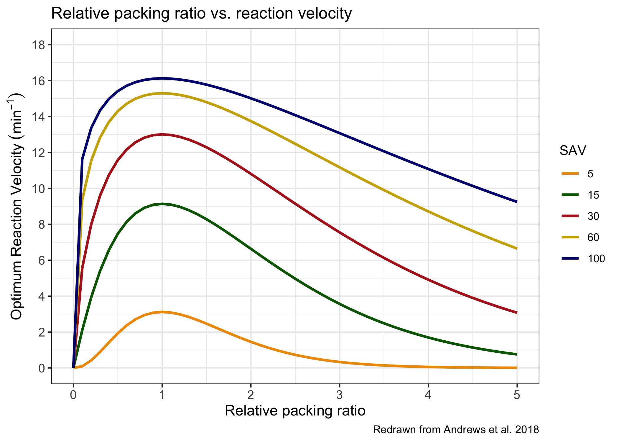
We’ll simulate the optimum reaction velocity from Rothermel (1972) and visualize how the behavior changes with fuel surface area to volume ratio (SAV) and relative packing ratio.

Optimum reaction velocity

Optimum reaction velocity (\(\Gamma'\), min\(^{-1}\)) is used to calculate reaction intensity (total heat release rate per unit area of fire front). Reaction velocity indicates the completeness and rate of fuel consumption, and optimum reaction velocity is the reaction velocity that would exist if the fuel were free of moisture and contained minerals at the same reaction concentration as alpha cellulose. It is calculated as:

\[ \Gamma' = \Gamma'_{max}\Big(\frac{\beta}{\beta_{op}}\Big)^A\exp(A(1 - \frac{\beta}{\beta_{op}}) \]

• \(A = 8.9033\sigma^{-0.7913}\)

• \(\Gamma'_{max}\): maximum reaction velocity (min\(^{-1}\))

• \(\frac{\beta}{\beta_{op}}\): relative packing ratio

• \(\sigma\): surface are to volume ratio (cm\(^{-1}\))

Based on the equation, optimum reaction velocity should increase with increasing SAV, and then possibly peak when relative packing ratio is 1.0. Below is a figure redrawn from a manuscript describing these relationships.

Exercise 4.1 Run a functional test

Below is a little test we can use to check out the function. Run the test and compare to the figure above.

from fire_model import FireEquations
import numpy as np
import matplotlib.pyplot as plt

def functional_test_optimum_velocity():
    """Functional test: plot relative packing ratio vs. reaction velocity."""
    sav_values = [5, 15, 30, 60, 100]
    beta_ratios = np.linspace(0.1, 5, 100)

    plt.figure(figsize=(8, 6))

    for sav in sav_values:
        max_vel = FireEquations.maximum_reaction_velocity(sav)
        velocities = [
            FireEquations.optimum_reaction_velocity(max_vel, sav, beta)
            for beta in beta_ratios
        ]
        plt.plot(beta_ratios, velocities, label=sav)

    plt.xlabel("Relative packing ratio")
    plt.ylabel("Optimum Reaction Velocity (min$^{-1}$)")
    plt.legend(loc="center left", bbox_to_anchor=(1, 0.5),
               title="SAV")
    plt.grid(True)

# TODO: run the functional test

What do you notice about the curves? Do they match the figure?

Exercise 4.2. Diagnosing an error

Let’s check out the code for the optimum reaction function.

??FireEquations.optimum_reaction_velocity

---

Can you fix the function?

# TODO rewrite the function
# def fixed_optimum_reaction_velocity(max_vel, sav, beta_ratio)
# ...

After you fix the function, update the functional test to use your new method and re-run it. Does it look better now?

What We Just Did

• Functional tests don’t always need to assert True/False.

• They can visualize the behavior of a system and can reveal when equations are producing incorrect results

In real models like FATES, this same principle helps catch subtle numerical or logic errors before full simulations are run.

Looking Ahead

• What are some functional tests you can design for your home systems?

• What infrastructure would you need to design (if any) to accomplish this?